Finite window correction

Measurements of “waiting times” or “survival times” taken within a finite time interval require special statistical treatment to account for the bias towards short measurements introduced by the measurement itself. For mathematical details, see the manuscript in preparation (Beltran et. al., *in preparation*).

import multi_locus_analysis as mla
import multi_locus_analysis.finite_window as fw

print(fw.__doc__)

For correcting interior- and exterior-censored data

This module is designed to facilitate working with Markov processes which have
been observed over finite windows of time.

Suppose you wish to observe a process that switches between states A and B, and
observe the process over a window of time :math:`[0, T]`.

There will be two types of "observed" times, which we we call "interior times"
(those when the entire time spent in the state is observed) and "exterior
times" (the lengths spent in the state that we observed at the start/end point
of our window).

For example, suppose you are observing two fluorescent loci that are either in
contact (A) or not (B). If you measure for 5s, and the loci begin in contact,
come apart at time t=2s, and rejoin at time t=4s,

::

        A A A A A A B B B B B B A A A A
        | - - | - - | - - | - - | - - | -- | -- | ...
        |                             |
    t = 0s    1s    2s    3s    4s    5s


we would say that T = 5s, and you measured one "interior" time of length 2s,
and two exterior times, one of length 2s and one of length 1s (at the start and
end of the window, respectively).

When histogramming these times, we must apply a statistical correction to the
final histogram weights due to the effects of the finite observation window.

The distribution of the exterior times :math:`f_E(t)` is exactly equal to the
survival function of the actual distribution :math:`S(t) = 1 - \int_0^t f(s)
ds` normalized to equal one over the observation interval.
No functions are currently included that leverage this, since extracting
information from the survival function is likely only worth it if a large
fraction of your observations are exterior times.

On the other hand, the interior times distribution is given by :math:`f_I(t) =
f(t)(T - t)` for :math:`t\in[0,T]`. In order to plot the actual shape of
:math:`f(t)` with this biasing removed, we provide the cdf_exact_given_windows
function below.

A typical workflow is, given an array of interior times, :code:`t`, and an
array of the window sizes each time was observed within, :code:`w`, is to
extract the CDF exactly, then optionally convert that to a PDF to display a
regular histogram

.. code-block:: python

    >>> x, cdf = cdf_exact_given_windows(t, w, pad_left_at_x=0)
    >>> xp, pdf = bars_given_cdf(x, cdf)
    >>> confint = simultaneous_confint_from_cdf(0.05, len(t), x, cdf)
    >>> xc, confs = bars_given_confint(x, confint)
    >>> plt.plot(xp, pdf, 'k', xc, confs, 'r-.')

The remainder of the functions herein are related to extracting confidence
intervals for these distributional estimates.

For details of the derivation, see the Biophysical Journal paper in preparation
by Beltran and Spakowitz.

We quickly set up some plotting defaults.

from bruno_util.plotting import use_cell_style
import matplotlib as mpl
figure_size = use_cell_style(mpl.rcParams)

# # Some helper code for getting new figsize if I change my mind about aspect ratio

# desired_aspect_ratio = (3/4)

# figwidth = fig.get_figwidth()
# figheight = fig.get_figheight()
# ax_bbox = ax.get_position()
# ax_width = ax_bbox.width*figwidth
# ax_height = ax_bbox.height*figheight


# ax_height_desired = ax_width*desired_aspect_ratio
# fig_height_desired = figheight + (ax_height_desired - ax_height)

# print(fig_height_desired)

Tutorial

Generating AB Trajectories

First let’s simply define two random variables to correspond to the “true” A and B waiting times. For convenience, we package them together with metadata that will be helpful for making pretty plots below, but notice that the only thing we need is the rvs function for each variable to perform the simulations.

from multi_locus_analysis.plotting import Variable
from scipy.stats import beta
import seaborn as sns

# for Beta distributions, making the window size a little less than 1 guarantees there's not too many,
# and also not too few waits per trajectory, so that the effect we want to show is visible
example_window = 0.8

wait_vars = [
    Variable(beta(5, 2),
             name='Beta(5, 2)',
             pretty_name=r'Beta$(\alpha{}=5, \beta{}=2)$',
             linestyle=':',
             color=sns.color_palette('colorblind')[2]),
    Variable(beta(2, 2),
             name='Beta(2, 2)',
             pretty_name=r'Beta$(\alpha{}=2, \beta{}=2)$',
             linestyle='--',
             color=sns.color_palette('colorblind')[3])
]

km_color = sns.color_palette('colorblind')[0]
interior_color = sns.color_palette('colorblind')[1]
interior_linestyle = '-.'

We use the :func:multi_locus_analysis.finite_window.ab_window function to generate example data:

print(fw.ab_window.__doc__)

Simulate an asynchronous two-state system from time 0 to `window_size`.

    Similar to :func:`multi_locus_analysis.finite_window.ab_window_fast`, but
    designed to work when the means of the distributions being used are hard to
    calculate.

    Simulate asynchronicity by starting the simulation in a uniformly random
    state at a time :math:`-t_\infty` (a large negative number).

    .. note::

        This number must be specified in the `offset` parameter and if it is
        not much larger than the means of the waiting times being used, the
        asynchronicity approximation will be very poor.

    The simulation only records between times 0 and window_size.

    Parameters
    ----------
    rands : (2,) List[scipy.stats.rv_continuous]
        Callable that takes "random_state" and "size" kwargs that accept
        a np.random.RandomState seed and a tuple specifying array sizes, resp.
    window_size : float
        The width of the window over which the observation takes place
    offset : float
        The (negative) time at which to start (in state 0) in order to
        equilibrate the simulation state by time t=0.
    states : (2,) array_like
        the "names" of each state, default to [0,1]
    num_replicates : int
        Number of times to run the simulation, default 1.
    seed : Optional[int]
        Random seed to start the simulation with
    random_state : np.random.RandomState
        Random state to start the simulation with. Preempts the seed argument.

    Returns
    -------
    df : pd.DataFrame
        The start/end times of each waiting time simulated. This data frame has
        columns=['replicate', 'state', 'start_time', 'end_time',
        'window_start', 'window_end'].

# trajs = fw.ab_window_fast(
#     [var.rvs for var in wait_vars],
#     means=[var.mean() for var in wait_vars],
#     window_size=example_window,
#     num_replicates=100_000,
#     states=[var.name for var in wait_vars]
# )
# trajs.head()

# We get the same result from the "fast" simulator, so don't use this.
import numpy as np

trajs = fw.ab_window(
    [var.rvs for var in wait_vars],
    window_size=example_window,
    offset=-100*np.sum([var.mean() for var in wait_vars]),
    num_replicates=100_000,
    states=[var.name for var in wait_vars]
)
trajs.head()

	replicate	state	start_time	end_time	window_start	window_end
0	0	Beta(5, 2)	-0.555918	0.415601	0	0.8
1	0	Beta(2, 2)	0.415601	0.684211	0	0.8
2	0	Beta(5, 2)	0.684211	1.447735	0	0.8
3	1	Beta(5, 2)	-0.202188	0.501101	0	0.8
4	1	Beta(2, 2)	0.501101	0.885911	0	0.8

From each trajectory, we can extract the wait times:

waits = fw.sim_to_obs(trajs)

waits['wait_type'] = waits['wait_type'].astype(str)

waits.head()

		state	start_time	end_time	wait_time	window_size	num_waits	wait_type
replicate	rank_order
0	1	Beta(5, 2)	0.000000	0.415601	0.415601	0.8	3	left exterior
	2	Beta(2, 2)	0.415601	0.684211	0.268610	0.8	3	interior
	3	Beta(5, 2)	0.684211	0.800000	0.115789	0.8	3	right exterior
1	1	Beta(5, 2)	0.000000	0.501101	0.501101	0.8	2	left exterior
	2	Beta(2, 2)	0.501101	0.800000	0.298899	0.8	2	right exterior

# # we can get the same result but vectorized, don't do this
# waits = trajs \
#     .groupby('replicate') \
#     .apply(fw.traj_to_waits)
# del waits['replicate']
# waits.head()

Naive histograms and Meier Kaplan

First, let’s evaluate the two ways that someone new to data censorship might guess would work. One could not be blamed for guessing that:

1. Just histogramming the interior times should work

2. Using the Meier-Kaplan correction (where the exterior times are considered “right-censored”) should work

There exist nice packages for computing the Meier-Kaplan estimator:

import lifelines
kmfs = {
    name: lifelines.KaplanMeierFitter() \
    .fit(state['wait_time'].values,
         event_observed=(state['wait_type'] == 'interior').values,
         label='Meier-Kaplan Estimator, $\pm$95% conf int')
    for name, state in waits.groupby('state')
}

Now we can compare these two guesses for how to approximate the “real” CDF against the ground truth. In order to be as generous as possible, we even normalize the two estimators so that they exactly match the ground truth at the window size, \(t = T\).

import matplotlib.pyplot as plt
import numpy as np
fig = plt.figure(
    figsize=figure_size['two-by-half column, four legend entries above'],
    constrained_layout=True
)
axs = fig.subplot_mosaic([[var.name for var in wait_vars]])
T = waits.window_size.max()
for var in wait_vars:
    # lifelines insists on returning a new Axes object....
    km_l = mpl.lines.Line2D([], [], color=km_color, label='Kaplan-Meier')
    ax = kmfs[var.name].plot_cumulative_density(
        color=km_color, ax=axs[var.name]
    )

    # plot actual distribution
    t = np.linspace(0, T, 100)
    analytical_l,  = ax.plot(
        t, var.cdf(t), color='k', label='Actual CDF'
    )

    # now compute the empirical distribution of the "interior" times
    interior = waits.loc[
        (waits['state'] == var.name) & (waits['wait_type'] == 'interior'),
        'wait_time'
    ].values
    x, cdf = fw.ecdf(interior, pad_left_at_x=0)

    interior_l, = ax.plot(
        x, cdf*var.cdf(x[-1]), c=var.color, ls=interior_linestyle,
        label='"Interior" eCDF'
    )

    # prettify the plot
    ax.set_xlim([0, waits.window_size.max()])
    ax.set_ylim([0, 1])
    ax.set_xlabel('time')
    ax.set_ylabel(r'Cumulative probability')

    # an empty handle acts effectively as a legend "title"
#     empty_handle = mpl.patches.Patch(alpha=0, label=var.pretty_name)
    legend = ax.legend(
        title=var.pretty_name,
        handles=[interior_l, km_l, analytical_l],
        # align bottom of legend 2% ax height above axis, filling full axis width
        bbox_to_anchor=(0., 1.02, 1., .102), loc='lower left',
        ncol=1, mode="expand", borderaxespad=0.
    )
#     legend.get_texts()[0].set_ha('right')
#     legend.get_texts()[0].set_position((-160, 0))

/home/bbeltr1/.miniconda3/envs/finite_window/lib/python3.8/site-packages/pandas/plotting/_matplotlib/tools.py:400: MatplotlibDeprecationWarning:
The is_first_col function was deprecated in Matplotlib 3.4 and will be removed two minor releases later. Use ax.get_subplotspec().is_first_col() instead.
  if ax.is_first_col():
/home/bbeltr1/.miniconda3/envs/finite_window/lib/python3.8/site-packages/pandas/plotting/_matplotlib/tools.py:400: MatplotlibDeprecationWarning:
The is_first_col function was deprecated in Matplotlib 3.4 and will be removed two minor releases later. Use ax.get_subplotspec().is_first_col() instead.
  if ax.is_first_col():

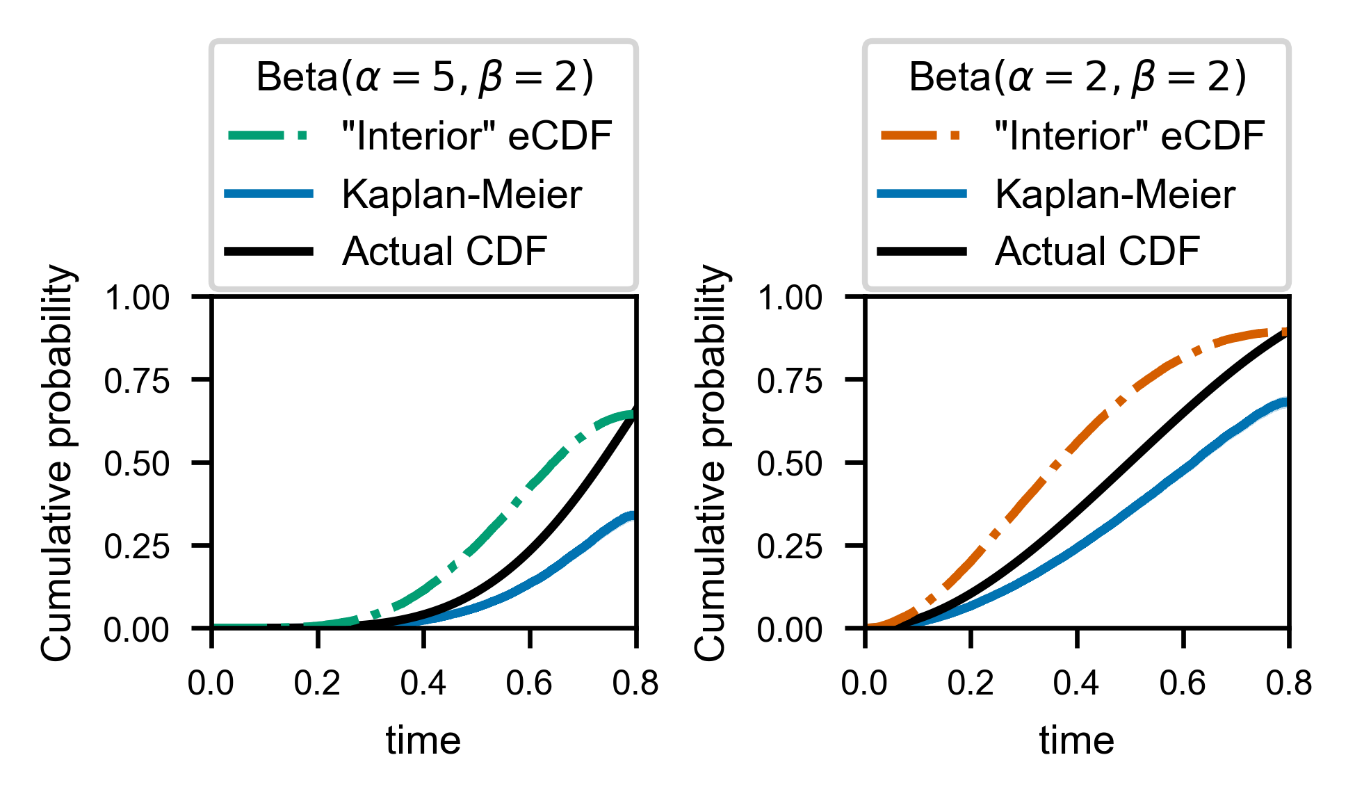
As far as I can tell at the time of writing this (end of 2020), the most commonly applied solution to this problem in the literature is in fact to use the “Kaplan-Meier” correction, which can be seen above (in blue, along with 95% (pointwise) confidence bands) to perform as poorly as the naive histogramming approach.

Why does this tried and tested technique for handling right-censored data fail? If the interval of observation is large enough that multiple state changes can be observed in one trajectory, then it can be shown that the Kaplan-Meier correction will under-correct, because there is negative autocorrelation between “successful” observation of times within a given trajectory (i.e. if we observe a long time, then we will be near to the end of our observation window, so the next observation must be small). The Meier-Kaplan correction was designed to work with right-censored data, but only with right-censored data where every single observed wait time is perfectly independent.

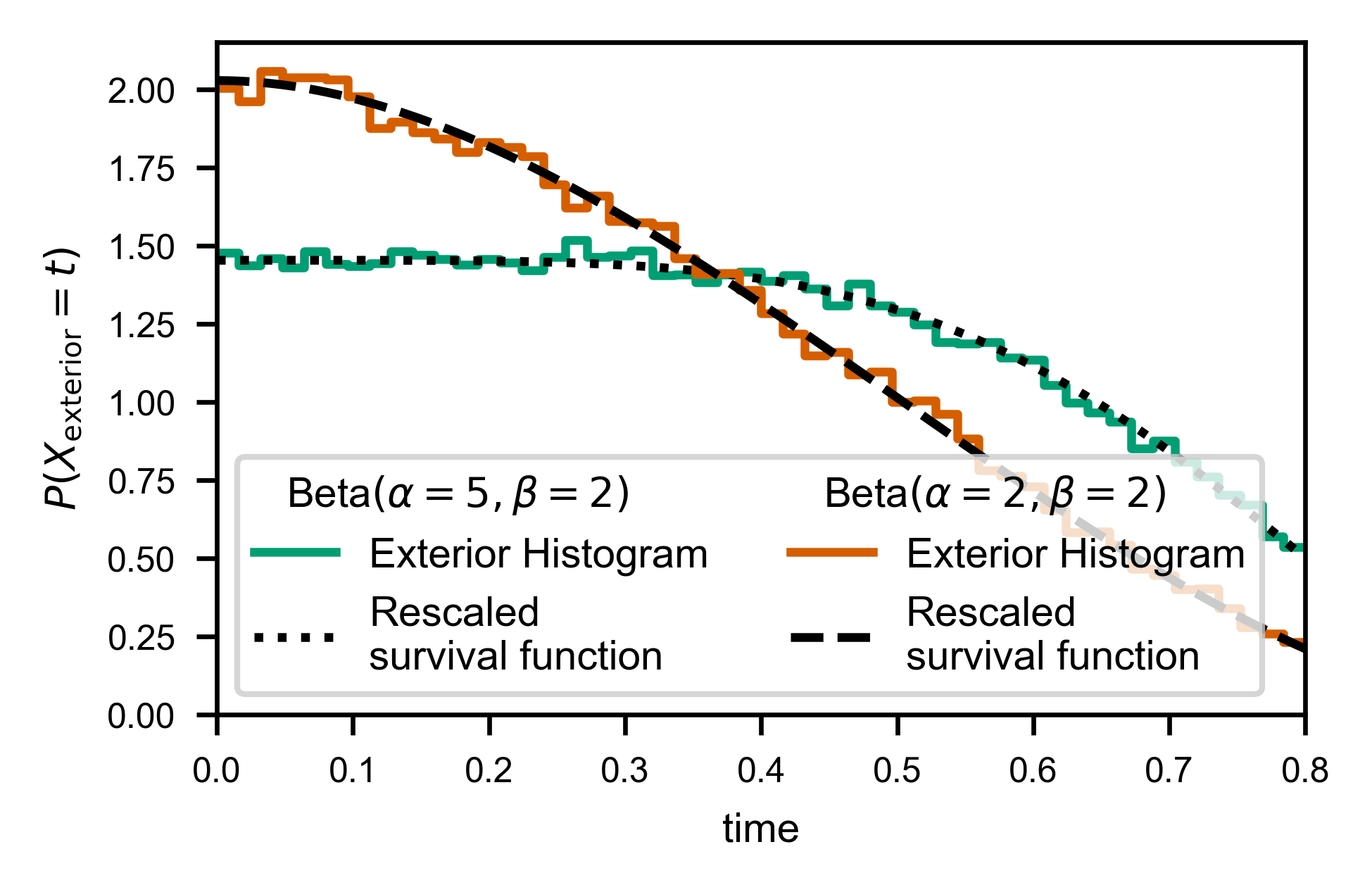
Exterior Times to Survival function

In order to correctly reproduce the actual underlying distribution, we must instead explicitly handle the “exterior censored” and “interior censored” times specially.

The exterior times are easy, as it can be shown (see “Theoretical Details” section below) that the probability distribution of the exterior times is exactly the survival function of the true waiting time distributions, normalized to one:

import scipy

fig, ax = plt.subplots(
    figsize=figure_size['full column'],
    constrained_layout=True
)
legend_entries = {var.name: [mpl.patches.Patch(alpha=0, label=var.pretty_name)]
                  for var in wait_vars}
T = waits.window_size.max()

for var in wait_vars:
    exterior = waits.loc[
        (waits['state'] == var.name) & (waits['wait_type'] != 'interior') \
        & (waits['wait_type'] != 'full exterior'),
        ['wait_time', 'window_size']
    ]

    t_bins = np.linspace(0, np.max(exterior.window_size), 51)
    dt = np.diff(t_bins)
    y, t_bins = np.histogram(
        exterior.wait_time.values,
        bins=t_bins
    )
    y = y/dt/len(exterior.wait_time)
    X, Y = mla.stats.bars_given_hist(y, t_bins)
    line, = ax.plot(X, Y, c=var.color, label='Exterior Histogram')
    legend_entries[var.name].append(line)

    t = np.linspace(0, T, 100)
    scale = T - scipy.integrate.quad(var.cdf, 0, T)[0]
    line, = ax.plot(t, var.sf(t)/scale, c='k', ls=var.linestyle,
                    label='Rescaled\nsurvival function')
    legend_entries[var.name].append(line)


ax.set_xlabel('time')
ax.set_ylabel(r'$P(X_\mathrm{exterior} = t)$')
ax.set_xlim([0, T])
ax.set_ylim([0, ax.get_ylim()[1]])

handles = [h for _, patches in legend_entries.items() for h in patches]
legend = ax.legend(handles=handles, ncol=2)
    # align bottom of legend 2% ax height above axis, filling full axis width
#     bbox_to_anchor=(0., 1.02, 1., .102), loc='lower left',
#     ncol=1, mode="expand", borderaxespad=0.
# )
# hack to left-align my "fake" legend column "titles"
for vpack in legend._legend_handle_box.get_children():
    for hpack in vpack.get_children()[:1]:
        hpack.get_children()[0].set_width(0)

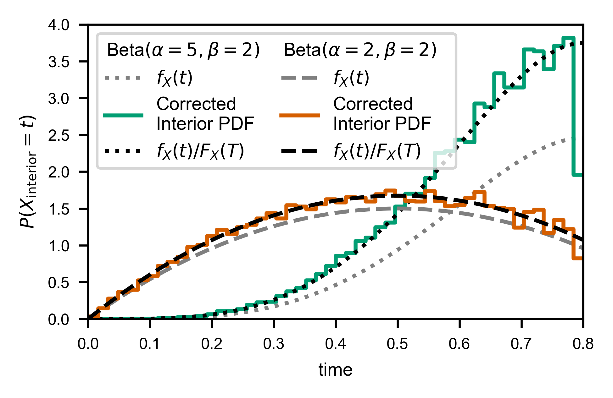
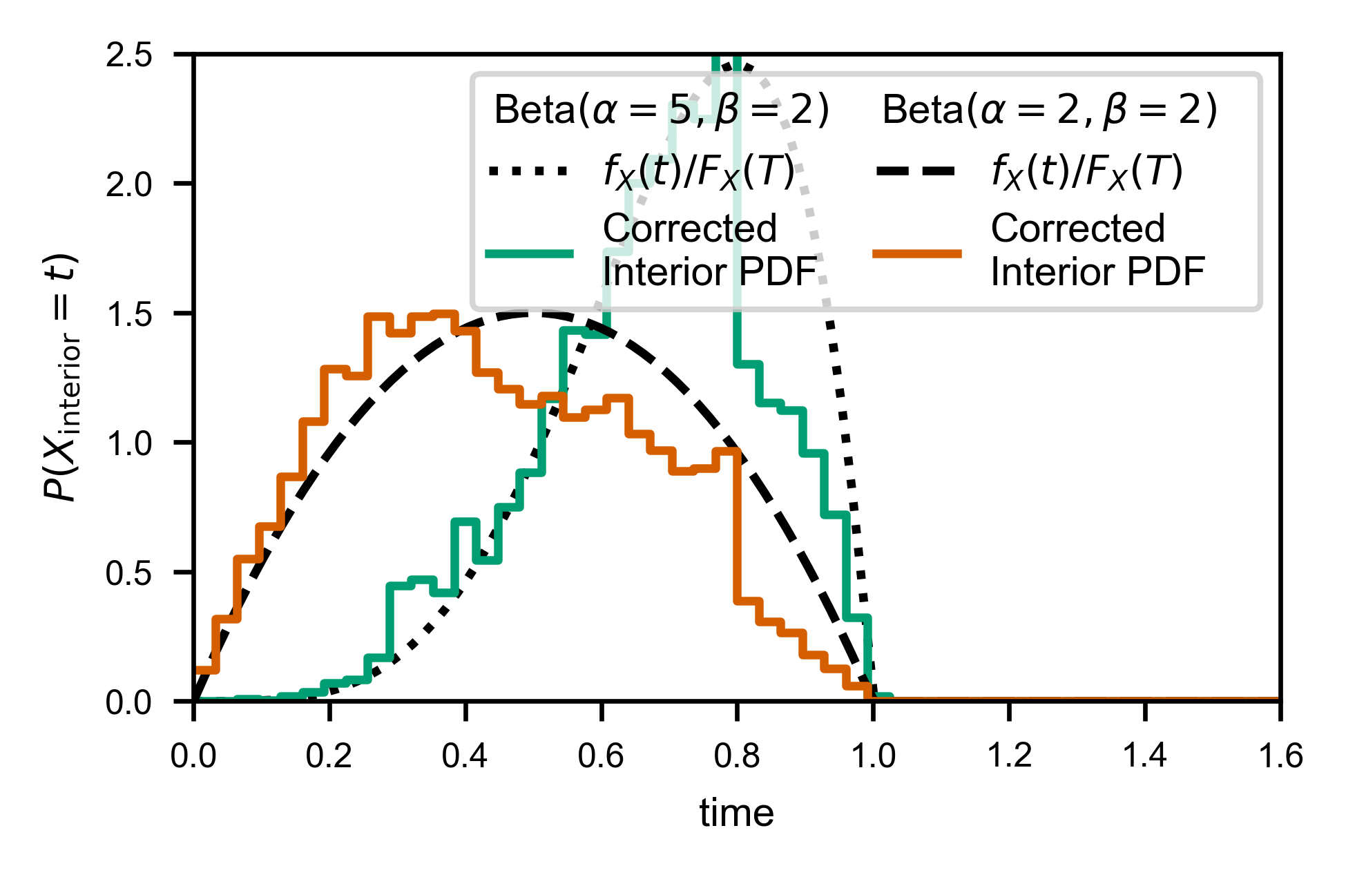
Interior Times to Likelihood

To handle the interior times, we need simply weight each observed time \(t_i\) by \(1/(T - t_i)\), which can easily be accomplished using np.histogram. (See “Theoretical Details” section below for justification).

Because we only observe times up to \(t=T\), we will actually be estimating:

\[\hat{f}_X(t) \approx P(X = t | X \leq T) = f_X(t) / F_X(T)\]

where \(\hat{f}\) is our corrected histogram, and \(f_X\) and \(F_X\) denote the probability distribution function (PDF) and cumulative distribution functions (CDF) of the random variable \(X\), respectively.

fig, ax = plt.subplots(
    figsize=figure_size['full column'],
    constrained_layout=True
)

legend_entries = {var.name: [mpl.patches.Patch(alpha=0, label=var.pretty_name)]
                  for var in wait_vars}
T = waits.window_size.max()
for var in wait_vars:
    line, = ax.plot(t, var.pdf(t), ls=var.linestyle,
                    c='0.5', label=f'$f_X(t)$')
    legend_entries[var.name].append(line)

    interior = waits.loc[
        (waits['state'] == var.name) & (waits['wait_type'] == 'interior'),
        ['wait_time', 'window_size']
    ].copy()
    interior['correction'] = 1/(interior.window_size - interior.wait_time)

    t_bins = np.linspace(0, T, 51)
    dt = np.diff(t_bins)
    y, t_bins = np.histogram(
        interior.wait_time.values,
        weights=interior.correction / np.sum(interior.correction),
        bins=t_bins
    )
    y = y / dt
    X, Y = mla.stats.bars_given_hist(y, t_bins)
    line, = ax.plot(X, Y, c=var.color, label='Corrected\nInterior PDF')
    legend_entries[var.name].append(line)

    t = np.linspace(0, T, 100)
    line, = ax.plot(t, var.pdf(t)/var.cdf(T),
                    c='k', ls=var.linestyle, label=f'$f_X(t)/F_X(T)$')
    legend_entries[var.name].append(line)

ax.set_xlabel('time')
ax.set_ylabel(r'$P(X_\mathrm{interior} = t)$')
ax.set_xlim([0, T])
ax.set_ylim([0, 4])
handles = [h for _, patches in legend_entries.items() for h in patches]
legend = ax.legend(handles=handles, ncol=2, columnspacing=0.5)

# hack to left-align my "fake" legend column "titles"
for vpack in legend._legend_handle_box.get_children():
    for hpack in vpack.get_children()[:1]:
        hpack.get_children()[0].set_width(0)
# even after the hack, need to move them over to "look" nice
legend.get_texts()[0].set_position((-40/600*mpl.rcParams['figure.dpi'], 0))
legend.get_texts()[4].set_position((-40/600*mpl.rcParams['figure.dpi'], 0))

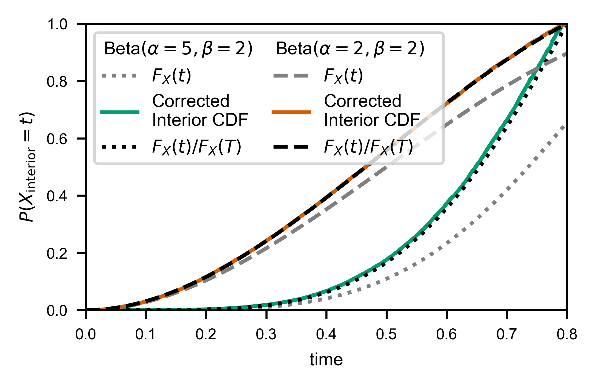
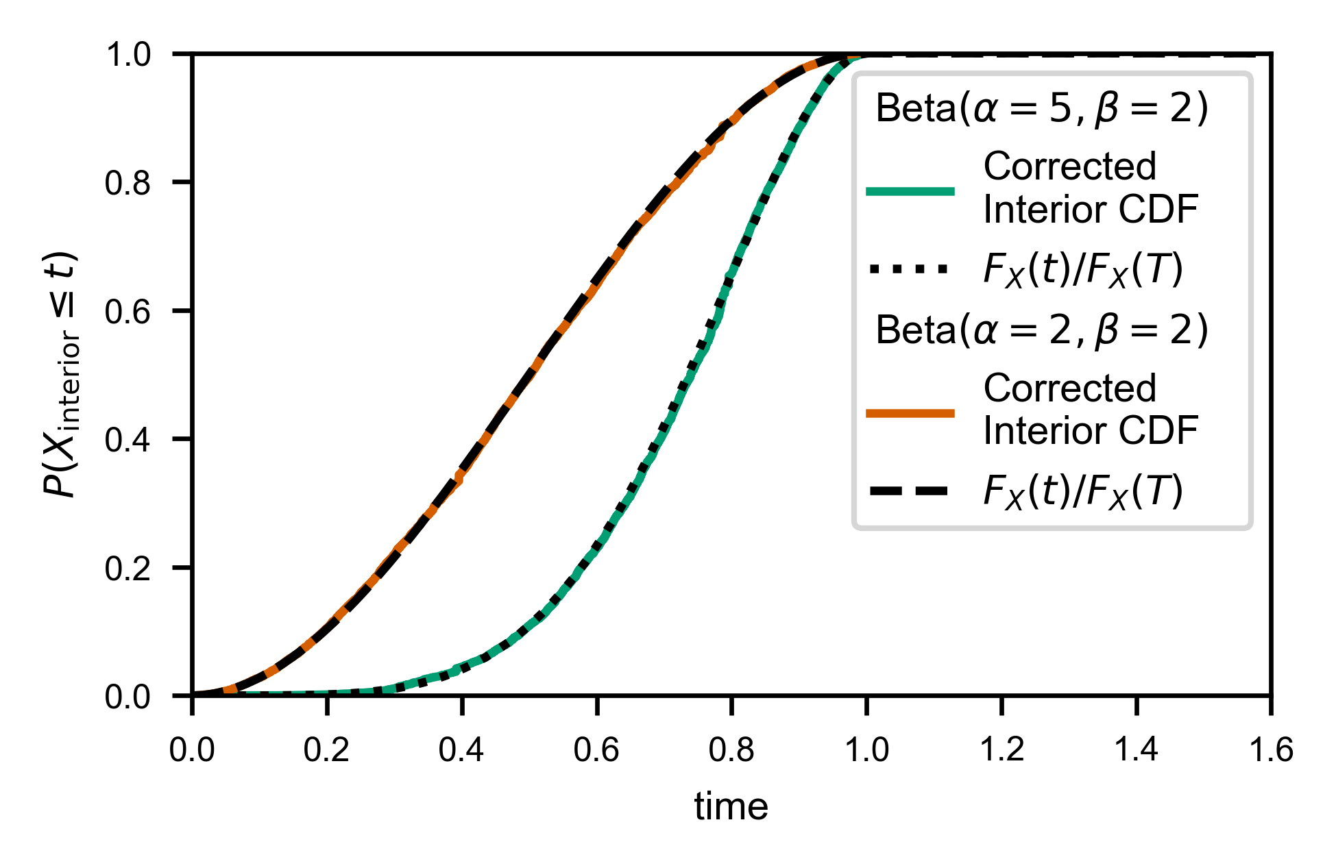
In order to facilitate applying the weights and normalizing correctly for performing the same correction without binning (e.g. to calculate the CDF), you can use the convenience function fw.ecdf_windowed:

print(fw.ecdf_windowed.__doc__)

    Empirical cumulative distribution for windowed observations.

    Parameters
    ----------
    times : (N,) array_like
        "Interior" waiting times.
    window_sizes : float or (N,) array_like
        The window size used. If a single value is passed, the window size is
        assumed to be constant.
    times_allowed : (M,) array_like
        Unique values that the data can take. Mostly useful for adding
        eCDF values at locations where data could or should have been observed
        but none was recorded (e.g. if a movie was taken with a given framerate
        but not all possible window lengths were observed).
    auto_pad_left : bool
        Deprecated. It makes more sense to default to left padding at zero for
        a renewal process. If left False, the data will not have a data value
        at the point where the eCDF equals zero. Use mean inter-data spacing to
        automatically generate an aesthetically reasonable such point. You
        *must* pass ``pad_left_at_x=False`` manually for this to work as
        expected.
    pad_left_at_x : float, default: 0
        Same as ``auto_pad_left``, but specify the point at which to add
        the leftmost point.
    window_sf : (M,) array_like of float
        For each unique window size in *window_sizes*, the number of
        trajectories with *at least* that window size. If not specified, it is
        assumed that each unique value of window size correponds to a unique
        trajectory. For the case of constant window size, this option is
        ignored.

    Returns
    -------
    x : (M,) array_like
        The values at which the eCDF was computed. By default
        :code:`np.sort(np.unique(y))`.
    cdf : (M,) array_like
        Values of the eCDF at each x.

    Notes
    -----
    If using ``times_allowed``, the *pad_left* parameters are redundant.

fig, ax = plt.subplots(
    figsize=figure_size['full column'],
    constrained_layout=True
)

legend_entries = {var.name: [mpl.patches.Patch(alpha=0, label=var.pretty_name)]
                  for var in wait_vars}
T = waits.window_size.max()
for var in wait_vars:
    line, = ax.plot(t, var.cdf(t), ls=var.linestyle,
                    c='0.5', label='$F_X(t)$')
    legend_entries[var.name].append(line)

    interior = waits.loc[
        (waits['state'] == var.name) & (waits['wait_type'] == 'interior'),
        ['wait_time', 'window_size']
    ].copy()
    x, cdf = fw.ecdf_windowed(
        interior.wait_time.values,
        interior.window_size.values,
        pad_left_at_x=0
    )
    line, = ax.plot(x, cdf, c=var.color, label='Corrected\nInterior CDF')
    legend_entries[var.name].append(line)

    t = np.linspace(0, T, 100)
    line, = ax.plot(t, var.cdf(t)/var.cdf(T), c='k', ls=var.linestyle, label='$F_X(t)/F_X(T)$')
    legend_entries[var.name].append(line)

ax.set_xlabel('time')
ax.set_ylabel(r'$P(X_\mathrm{interior} = t)$')
ax.set_xlim([0, T])
ax.set_ylim([0, 1])
handles = [h for _, patches in legend_entries.items() for h in patches]
legend = ax.legend(handles=handles, ncol=2, columnspacing=0.5)

# hack to left-align my "fake" legend column "titles"
for vpack in legend._legend_handle_box.get_children():
    for hpack in vpack.get_children()[:1]:
        hpack.get_children()[0].set_width(0)
# even after the hack, need to move them over to "look" nice
legend.get_texts()[0].set_position((-40/600*mpl.rcParams['figure.dpi'], 0))
legend.get_texts()[4].set_position((-40/600*mpl.rcParams['figure.dpi'], 0))

Interior and Exterior times to “real” distribution

Typically, a likelihood estimate like \(\hat{F}\) or \(\hat{f}\) is sufficient to do parameter estimation, or at least to get a sense of the shape of the distribution. (For example, to determine the power-law or exponential rate of your system, simply plot this likelihood on a log-log or semi-log scale, respectively, and the constant factor will not affect the estimation).

On the other hand, there are times where it is important to know exactly how much contribution comes from waiting times that are greater than the observation window. In these cases, we can estimate \(F_X(T)\) to get a correctly normalized estimate of the ground truth.

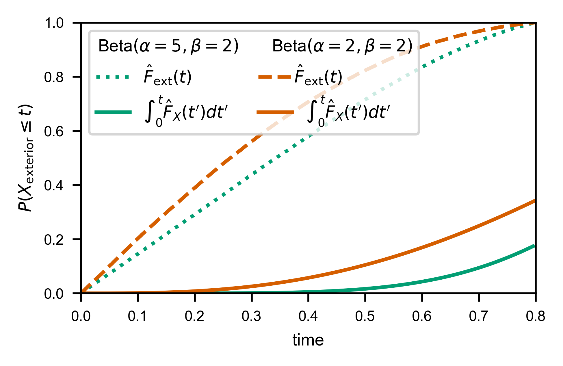
There are many ways to estimate this quantity (see “Theoretical Details” section for more), but the most numerically stable one I have found so far is to notice that we have two indepedent ways of computing a function that corresponds to a uniform linear scaling of \(F_X(t)\):

1. Histogram of exterior times \(\propto S_X(t)\). Let’s call it \(\hat{f}_\text{ext}(t) = S_X(t) / Z_X\).

2. The corrected interior times CDF is given by \(\hat{F}_X(t) = F_X(t) / F_X(T)\).

So we could in principle divide the height of the last histogram bar by the height of the first histogram bar (since we know \(S_X(0)=1\)) to get \(S_X(T) = 1 - F_X(T)\), but this operation is very sensitive to our choice of histogram binning, and quite noisy.

Instead, we notice \(\hat{f}_\text{ext}(t) = a + b*\hat{F}_X(t)\), where \(a = 1/Z_X\) and \(b = -F_X(T)/Z_X\), so we simply find the \(a\) and \(b\) which minimize the error

\[\| \hat{f}_\text{ext}(t) - \left(a + b*\hat{F}_X(t) \right) \|_2,\]

then compute \(F_X(T) \approx -b/a\).

In fact, to prevent binning artifacts from the fact that \(\hat{f}_\text{ext}(t)\) is computed via a histogram, we can instead use the empirical CDF of the exterior times, and minimize:

\[\| \hat{f}_\text{ext}(t) - \left(t a + b*\int_0^t \hat{F}_X(t') dt' \right) \|_2.\]

fig, ax = plt.subplots(
    figsize=figure_size['full column'],
    constrained_layout=True
)

legend_entries = {var.name: [mpl.patches.Patch(alpha=0, label=var.pretty_name)]
                  for var in wait_vars}
T = waits.window_size.max()
for var in wait_vars:
    interior = waits.loc[
        (waits['state'] == var.name) & (waits['wait_type'] == 'interior'),
        ['wait_time', 'window_size']
    ].copy()
    x_int, cdf_int = fw.ecdf_windowed(
        interior.wait_time.values,
        interior.window_size.values,
        pad_left_at_x=0
    )
    # now compute integral of CDF w.r.t.
    cdf_mid = (cdf_int[1:] + cdf_int[:-1]) / 2
    int_cdf = np.zeros_like(cdf_int)
    int_cdf[1:] = np.cumsum(cdf_mid * np.diff(x_int))

    exterior = waits.loc[
        (waits['state'] == var.name) & (waits['wait_type'] != 'interior') \
        & (waits['wait_type'] != 'full exterior'),
        ['wait_time', 'window_size']
    ]
    x_ext, cdf_ext = fw.ecdf(
        exterior.wait_time.values,
        pad_left_at_x=0
    )

    line, = ax.plot(x_ext, cdf_ext, c=var.color, ls=var.linestyle,
                    label='$\hat{F}_\mathrm{ext}(t)$')
    legend_entries[var.name].append(line)

    line, = ax.plot(x_int, int_cdf, c=var.color, ls='-',
                    label="$\int_0^t \hat{F}_X(t')dt'$")
    legend_entries[var.name].append(line)

ax.set_xlabel('time')
ax.set_ylabel(r'$P(X_\mathrm{exterior} \leq t)$')
ax.set_xlim([0, T])
ax.set_ylim([0, 1])
handles = [h for _, patches in legend_entries.items() for h in patches]
legend = ax.legend(handles=handles, loc='upper left', ncol=2, columnspacing=0.5)

# hack to left-align my "fake" legend column "titles"
for vpack in legend._legend_handle_box.get_children():
    for hpack in vpack.get_children()[:1]:
        hpack.get_children()[0].set_width(0)
# even after the hack, need to move them over to "look" nice
legend.get_texts()[0].set_position((-40/600*mpl.rcParams['figure.dpi'], 0))
legend.get_texts()[4].set_position((-40/600*mpl.rcParams['figure.dpi'], 0))

cdf_int_to_ext_cdf = {}

Now we compute the estimate:

fig, ax = plt.subplots(
    figsize=figure_size['full column'],
    constrained_layout=True
)

legend_entries = {var.name: [mpl.patches.Patch(alpha=0, label=var.pretty_name)]
                  for var in wait_vars}
T = waits.window_size.max()
for var in wait_vars:
    interior = waits.loc[
        (waits['state'] == var.name) & (waits['wait_type'] == 'interior'),
        ['wait_time', 'window_size']
    ].copy()
    x_int, cdf_int = fw.ecdf_windowed(
        interior.wait_time.values,
        interior.window_size.values,
        pad_left_at_x=0
    )
    # now compute integral of CDF w.r.t.
    cdf_mid = (cdf_int[1:] + cdf_int[:-1]) / 2
    int_cdf = np.zeros_like(cdf_int)
    int_cdf[1:] = np.cumsum(cdf_mid * np.diff(x_int))

    exterior = waits.loc[
        (waits['state'] == var.name) & (waits['wait_type'] != 'interior') \
        & (waits['wait_type'] != 'full exterior'),
        ['wait_time', 'window_size']
    ]
    x_ext, cdf_ext = fw.ecdf(
        exterior.wait_time.values,
        pad_left_at_x=0
    )

    t_all = np.sort(np.concatenate((x_int, x_ext)))
    resampled_int_cdf = np.interp(t_all, x_int, int_cdf)
    resampled_ext_cdf = np.interp(t_all, x_ext, cdf_ext)
    def err_f(ab, t, integrated_cdf, exterior_cdf):
        return np.linalg.norm(ab[0] * t + ab[1] * integrated_cdf - exterior_cdf)

    opt_out = scipy.optimize.minimize(
        err_f,
        x0=[1, -1],
        args=(t_all, resampled_int_cdf, resampled_ext_cdf),
        bounds=((0, np.inf), (-np.inf, 0)),
    )
    if not opt_out.success:
        raise ValueError("Unable to compute F_X(T)!")
    a, b = opt_out.x
    cdf_int_to_ext_cdf[var.name] = {'a': a, 'b': b}

    line, = ax.plot(x_ext, cdf_ext, c=0.7*np.array(var.color), ls=var.linestyle,
                    lw=1.5,
                    label='$\hat{F}_\mathrm{ext}(t)$')
    legend_entries[var.name].append(line)

    line, = ax.plot(x_int, a*x_int + b*int_cdf, c=var.color, ls='-',
                    lw=1,
                    label="$\int_0^t \hat{F}_X(t')dt'$")
    legend_entries[var.name].append(line)

ax.set_xlabel('time')
ax.set_ylabel(r'$P(X_\mathrm{exterior} \leq t)$')
ax.set_xlim([0, T])
ax.set_ylim([0, 1])
handles = [h for _, patches in legend_entries.items() for h in patches]
legend = ax.legend(handles=handles, loc='upper left', ncol=2, columnspacing=0.5)

# hack to left-align my "fake" legend column "titles"
for vpack in legend._legend_handle_box.get_children():
    for hpack in vpack.get_children()[:1]:
        hpack.get_children()[0].set_width(0)
# even after the hack, need to move them over to "look" nice
legend.get_texts()[0].set_position((-40/600*mpl.rcParams['figure.dpi'], 0))
legend.get_texts()[3].set_position((-40/600*mpl.rcParams['figure.dpi'], 0))

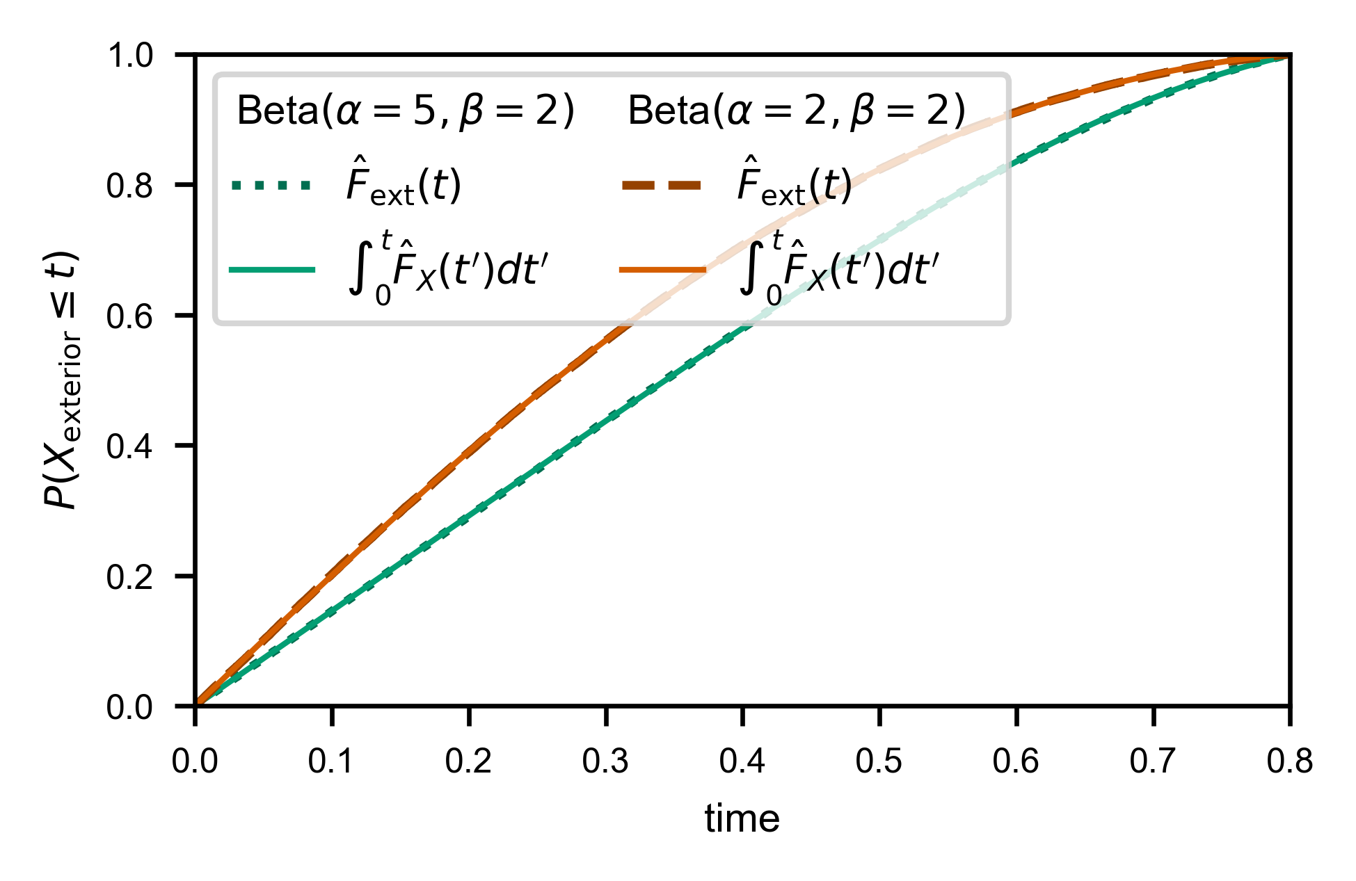
Here’s how well we are able to estimate \(Z_X\) and \(F_X(T)\) for this particular set of trajectories:

for var in wait_vars:
    a = cdf_int_to_ext_cdf[var.name]['a']
    b = cdf_int_to_ext_cdf[var.name]['b']
    T = waits.window_size.max()
    Z_X = T - scipy.integrate.quad(var.cdf, 0, T)[0]
    print(f'${1/a} \\approx {Z_X}$')
    print(f'${-b/a} \\approx {var.cdf(T)}$')

$0.6850002012834457 \approx 0.6876525714285715$
$0.6505871277146529 \approx 0.6553600000000002$
$0.49455460682752556 \approx 0.4927999999999999$
$0.8881117394216376 \approx 0.896$

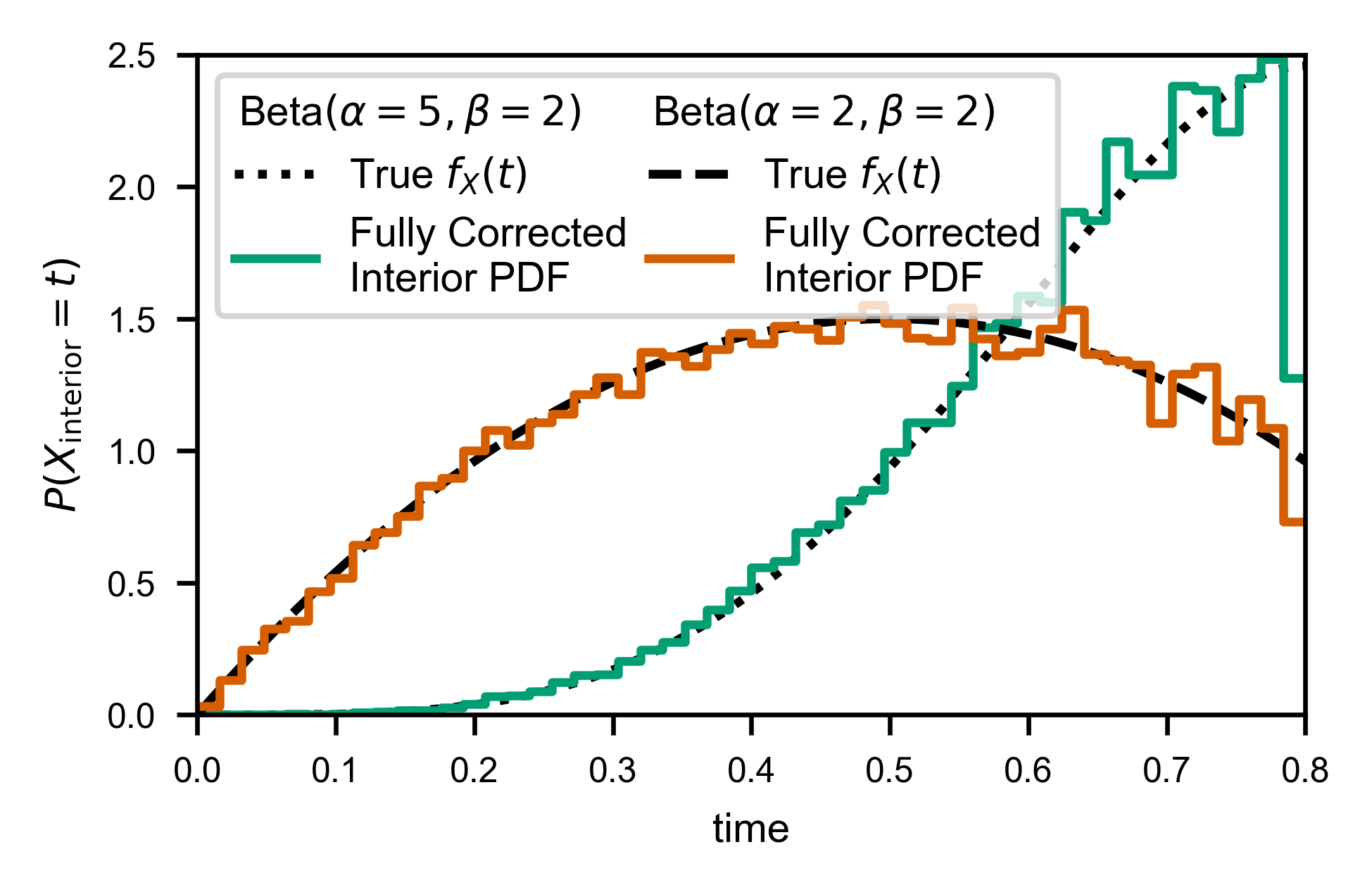
Now we can compute correctly normalized wait time distributions:

fig, ax = plt.subplots(
    figsize=figure_size['full column'],
    constrained_layout=True
)

legend_entries = {var.name: [mpl.patches.Patch(alpha=0, label=var.pretty_name)]
                  for var in wait_vars}
T = waits.window_size.max()
for var in wait_vars:
    line, = ax.plot(t, var.pdf(t), ls=var.linestyle,
                    c='k', label=f'True $f_X(t)$')
    legend_entries[var.name].append(line)

    interior = waits.loc[
        (waits['state'] == var.name) & (waits['wait_type'] == 'interior'),
        ['wait_time', 'window_size']
    ].copy()
    interior['correction'] = 1/(interior.window_size - interior.wait_time)

    t_bins = np.linspace(0, T, 51)
    dt = np.diff(t_bins)
    y, t_bins = np.histogram(
        interior.wait_time.values,
        weights=interior.correction / np.sum(interior.correction),
        bins=t_bins
    )
    y = y / dt
    X, Y = mla.stats.bars_given_hist(y, t_bins)
    a = cdf_int_to_ext_cdf[var.name]['a']
    b = cdf_int_to_ext_cdf[var.name]['b']
    line, = ax.plot(X, Y*(-b/a), c=var.color, label='Fully Corrected\nInterior PDF')
    legend_entries[var.name].append(line)

ax.set_xlabel('time')
ax.set_ylabel(r'$P(X_\mathrm{interior} = t)$')
ax.set_xlim([0, T])
ax.set_ylim([0, 2.5])
handles = [h for _, patches in legend_entries.items() for h in patches]
legend = ax.legend(handles=handles, ncol=2, columnspacing=0.5)

# hack to left-align my "fake" legend column "titles"
for vpack in legend._legend_handle_box.get_children():
    for hpack in vpack.get_children()[:1]:
        hpack.get_children()[0].set_width(0)
# even after the hack, need to move them over to "look" nice
legend.get_texts()[0].set_position((-40/600*mpl.rcParams['figure.dpi'], 0))
legend.get_texts()[3].set_position((-40/600*mpl.rcParams['figure.dpi'], 0))

Heterogeneous Window Size

For arbitrary collections of data measured with potentially different window sizes, we simply need to correct for the fraction of trajectories in which each time could have been observed at all.

import importlib
importlib.reload(fw.munging)
importlib.reload(fw)

<module 'multi_locus_analysis.finite_window' from '/home/bbeltr1/developer/multi_locus_analysis/multi_locus_analysis/finite_window/__init__.py'>

import numpy as np
import pandas as pd

# generate same distribution, but with three different window sizes
het_trajs = [
    fw.ab_window(
        [var.rvs for var in wait_vars],
        window_size=window,
        offset=-100*np.sum([var.mean() for var in wait_vars]),
        num_replicates=10_000,
        states=[var.name for var in wait_vars]
    )
    for window in np.array([1/2, 1, 2])*example_window
]
het_trajs = pd.concat(het_trajs, ignore_index=True)
# multi_T_waits = het_trajs \
#     .groupby(['window_end', 'replicate']) \
#     .apply(fw.traj_to_waits)
# del multi_T_waits['replicate']
# del multi_T_waits['window_end']
# multi_T_waits.head()

# replicate id only  unique given window size
multi_T_waits = fw.sim_to_obs(het_trajs, traj_cols=['window_end', 'replicate'])
# copying a column to gruopby is easier than the
# reset_index magic required for the below
multi_T_waits.head()

			state	start_time	end_time	wait_time	window_size	num_waits	wait_type
window_end	replicate	rank_order
0.4	0	1	Beta(5, 2)	0.000000	0.324731	0.324731	0.4	2	left exterior
		2	Beta(2, 2)	0.324731	0.400000	0.075269	0.4	2	right exterior
	1	1	Beta(5, 2)	0.000000	0.400000	0.400000	0.4	1	full exterior
	2	1	Beta(5, 2)	0.000000	0.344230	0.344230	0.4	2	left exterior
		2	Beta(2, 2)	0.344230	0.400000	0.055770	0.4	2	right exterior

Notice the only difference is that the weights also include the fraction of trajectories that can have even observed the given wait time in the first place.

fig, ax = plt.subplots(
    figsize=figure_size['full column'],
    constrained_layout=True
)

legend_entries = {var.name: [mpl.patches.Patch(alpha=0, label=var.pretty_name)]
                  for var in wait_vars}
T = multi_T_waits.window_size.max()
# get fraction of windows that are at *least* of each width
window_sizes, window_cumulant = mla.stats.ecdf(
    multi_T_waits.groupby(['window_end', 'replicate'])['window_size'].first().values,
    pad_left_at_x=0
)
window_frac_at_least = 1 - window_cumulant
for var in wait_vars:
    t = np.linspace(0, T, 100)

    line, = ax.plot(t, var.pdf(t)/var.cdf(T), ls=var.linestyle,
                    c='k', label=f'$f_X(t)/F_X(T)$')
    legend_entries[var.name].append(line)

    interior = multi_T_waits.loc[
        (multi_T_waits['state'] == var.name) & (multi_T_waits['wait_type'] == 'interior'),
        ['wait_time', 'window_size']
    ].copy()
    # for each observed time, we can get number of windows in which it can have been observed
    window_i = np.searchsorted(window_sizes, interior.wait_time) - 1
    frac_trajs_observable = window_frac_at_least[window_i]
    interior['correction'] = 1 / frac_trajs_observable / (interior.window_size - interior.wait_time)

    t_bins = np.linspace(0, T, 51)
    dt = np.diff(t_bins)
    y, t_bins = np.histogram(
        interior.wait_time.values,
        weights=interior.correction / np.sum(interior.correction),
        bins=t_bins
    )
    y = y / dt
    X, Y = mla.stats.bars_given_hist(y, t_bins)
    line, = ax.plot(X, Y, c=var.color, label='Incorrect\nInterior PDF')
    legend_entries[var.name].append(line)

ax.set_xlabel('time')
ax.set_ylabel(r'$P(X_\mathrm{interior} = t)$')
ax.set_xlim([0, T])
ax.set_ylim([0, 2.5])
handles = [h for _, patches in legend_entries.items() for h in patches]
legend = ax.legend(handles=handles, ncol=1, loc='upper right')

# hack to left-align my "fake" legend column "titles"
for vpack in legend._legend_handle_box.get_children():
    for i in [0, 3]:
        hpack = vpack.get_children()[i]
        hpack.get_children()[0].set_width(0)
# even after the hack, need to move them over to "look" nice
legend.get_texts()[0].set_position((-40/600*mpl.rcParams['figure.dpi'], 0))
legend.get_texts()[3].set_position((-40/600*mpl.rcParams['figure.dpi'], 0))

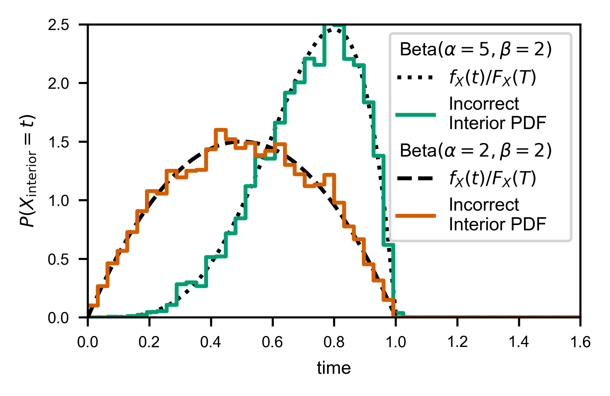
Here’s what it looks like if we don’t do the extra correction. Notice the “jumps” at each window size, due to the missing correction factor:

fig, ax = plt.subplots(
    figsize=figure_size['full column'],
    constrained_layout=True
)

legend_entries = {var.name: [mpl.patches.Patch(alpha=0, label=var.pretty_name)]
                  for var in wait_vars}
T = multi_T_waits.window_size.max()
for var in wait_vars:
    t = np.linspace(0, T, 100)

    line, = ax.plot(t, var.pdf(t)/var.cdf(T), ls=var.linestyle,
                    c='k', label=f'$f_X(t)/F_X(T)$')
    legend_entries[var.name].append(line)

    interior = multi_T_waits.loc[
        (multi_T_waits['state'] == var.name) & (multi_T_waits['wait_type'] == 'interior'),
        ['wait_time', 'window_size']
    ].copy()
    interior['correction'] = 1/(interior.window_size - interior.wait_time)

    t_bins = np.linspace(0, T, 51)
    dt = np.diff(t_bins)
    y, t_bins = np.histogram(
        interior.wait_time.values,
        weights=interior.correction / np.sum(interior.correction),
        bins=t_bins
    )
    y = y / dt
    X, Y = mla.stats.bars_given_hist(y, t_bins)
    line, = ax.plot(X, Y*(-b/a), c=var.color, label='Corrected\nInterior PDF')
    legend_entries[var.name].append(line)

ax.set_xlabel('time')
ax.set_ylabel(r'$P(X_\mathrm{interior} = t)$')
ax.set_xlim([0, T])
ax.set_ylim([0, 2.5])
handles = [h for _, patches in legend_entries.items() for h in patches]
legend = ax.legend(handles=handles, ncol=2, columnspacing=0.5)

# hack to left-align my "fake" legend column "titles"
for vpack in legend._legend_handle_box.get_children():
    for hpack in vpack.get_children()[:1]:
        hpack.get_children()[0].set_width(0)
# even after the hack, need to move them over to "look" nice
legend.get_texts()[0].set_position((-40/600*mpl.rcParams['figure.dpi'], 0))
legend.get_texts()[3].set_position((-40/600*mpl.rcParams['figure.dpi'], 0))

As you might expect, fw.ecdf_windowed takes a window_cumulant argument, to allow you to specify how many of each window type there are (since it’s not possible to infer that information purely from a list of interior times and corresponding window sizes).

If your window size is drawn randomly, then each window size is effectively unique, and the default value of window_cumulant=None will do the appropriate computation for you.

fig, ax = plt.subplots(
    figsize=figure_size['full column'],
    constrained_layout=True
)

legend_entries = {var.name: [mpl.patches.Patch(alpha=0, label=var.pretty_name)]
                  for var in wait_vars}
T = multi_T_waits.window_size.max()
window_sizes, window_cumulant = mla.stats.ecdf(
    multi_T_waits.groupby(['window_end', 'replicate'])['window_size'].first().values,
    pad_left_at_x=0
)
for var in wait_vars:
    t = np.linspace(0, T, 100)

    interior = multi_T_waits.loc[
        (multi_T_waits['state'] == var.name) & (multi_T_waits['wait_type'] == 'interior'),
        ['wait_time', 'window_size']
    ].copy()

    x, cdf = fw.ecdf_windowed(
        interior.wait_time, interior.window_size,
        pad_left_at_x=0, window_sf=(1 - window_cumulant)
    )
    line, = ax.plot(x, cdf, c=var.color, label='Corrected\nInterior CDF')
    legend_entries[var.name].append(line)

    line, = ax.plot(t, var.cdf(t)/var.cdf(T), ls=var.linestyle,
                    c='k', label=f'$F_X(t)/F_X(T)$')
    legend_entries[var.name].append(line)


ax.set_xlabel('time')
ax.set_ylabel(r'$P(X_\mathrm{interior} \leq t)$')
ax.set_xlim([0, T])
ax.set_ylim([0, 1])
handles = [h for _, patches in legend_entries.items() for h in patches]
legend = ax.legend(handles=handles, ncol=1, loc='upper right')

# hack to left-align my "fake" legend column "titles"
for vpack in legend._legend_handle_box.get_children():
    for i in [0, 3]:
        hpack = vpack.get_children()[i]
        hpack.get_children()[0].set_width(0)
# even after the hack, need to move them over to "look" nice
legend.get_texts()[0].set_position((-40/600*mpl.rcParams['figure.dpi'], 0))
legend.get_texts()[3].set_position((-40/600*mpl.rcParams['figure.dpi'], 0))

A Caveat for Discrete Movies

While we would ideally have an exact measurement of when transitions between A and B states happen, it is more often the case that we have a “movie” of sorts, where we measure the state of the system at a fixed set of frames.

This only provides us with upper and lower bounds for the actual waiting time that we’re trying to observe. For example, consider the trajectory depicted below.

    A A A A A B B B B B B B A A A A B
    | - - - | - - - | - - - | - - - |  ...
    |                               |
t = 0s      1s      2s      3s      4s

This trajectory, when measured at the discrete times shown, would look like

pd.Series({0: 'A', 1: 'A', 2: 'B', 3: 'A', 4: 'B'}).head()
    0    A
    1    A
    2    B
    3    A
    4    B
    dtype: object

Naively, if you only had this movie in front of you with no knowledge of the actual underlying state change times, it might seem to suggest that there was an exterior-censored “A” of length 2, one each interior censored times of length 1, and one exterior-censored “B” time of length 1. However, by looking at the true trajctory above, we see that the first “A” wait was much shorter than 2s, and the first “B” wait was much longer than 1s, whereas the last “A” wait just happened to match up with our prediction of 1s.

Because our normalization factor depends non-linearly on the observed waiting time, one might guess that simply using the “naive” times might cause bias. We will show that this is the case by generating some artificial movies ourselves.

Generating Discrete Trajectories (Movies)

multi_locus_analysis.finite_window includes a convenience method for generating “movie frames” from the output of the AB_window* functions:

print(fw.state_changes_to_movie_frames.__doc__)

    Convert state changes into discrete-time observations of state.

    Takes a Series of state change times into a Series containing
    observations at the times requested. The times become the index.

    Parameters
    ----------
    times : (N,) array_like
        times at which to "measure" what state we're in to make the new
        trajectories.
    traj : pd.DataFrame
        should have `state_col` and `start_times_col` columns. the values of
        `state_col` will be copied over verbatim.
    state_col : string
        name of column containing the state being transitioned out of for each
        measurement in `traj`.
    start_times_col : string
        name of column containing times at which `traj` changed state
    end_times_col : (optional) string
        by default, the function assumes that times after the last start time
        are in the same state. if passed, this column is used to determine at
        what time the last state "finished". times after this will be labeled
        as NaN.

    Returns
    -------
    movie : pd.Series
        Series defining the "movie" with frames taken at `times` that
        simply measures what state `traj` is in at each frame. index is
        `times`, `state_col` is used to name the Series.

    Notes
    -----
    A start time means that if we observe at that time, the state transition
    will have already happened (right-continuity). This is confusing in
    words, but simple to see in an example (see the example below).

    Examples
    --------
    For the DataFrame

        >>> df = pd.DataFrame([['A',  -1, 0.1], ['B', 0.1, 1.0]],
        >>>     columns=['state', 'start_time', 'end_time'])

    the discretization into tenths of seconds would give

        >>> state_changes_to_movie_frames(df, times=np.linspace(0, 1, 11),
        >>>     end_times_col='end_time')
        t
        0.0      A
        0.1      B
        0.2      B
        0.3      B
        0.4      B
        0.5      B
        0.6      B
        0.7      B
        0.8      B
        0.9      B
        1.0    NaN
        Name: state, dtype: object

    Notice in particular how at 0.1, the state is already 'B'. Similarly at
    time 1.0 the state is already "unknown". This is what is meant by the Notes
    section above.

    If the `end_times_col` argument is omitted, then the last observed state is
    assumed to continue for all `times` requested from then on:

        >>> state_changes_to_movie_frames(df, times=np.linspace(0, 1, 11))
        t
        0.0    A
        0.1    B
        0.2    B
        0.3    B
        0.4    B
        0.5    B
        0.6    B
        0.7    B
        0.8    B
        0.9    B
        1.0    B
        Name: state, dtype: object

This function has an alias for convenience: multi_locus_analysis.finite_window.traj_to_movie.

T = trajs.window_end.max()
movie_frame_t = np.linspace(0, T, 21)
movies = trajs.groupby('replicate').apply(
    fw.traj_to_movie,
    times=movie_frame_t
)
movies.head()

t	0.00	0.04	0.08	0.12	0.16	0.20	0.24	0.28	0.32	0.36	...	0.44	0.48	0.52	0.56	0.60	0.64	0.68	0.72	0.76	0.80
replicate
0	Beta(2, 2)	Beta(2, 2)	Beta(2, 2)	Beta(2, 2)	Beta(2, 2)	Beta(2, 2)	Beta(2, 2)	Beta(2, 2)	Beta(2, 2)	Beta(2, 2)	...	Beta(2, 2)	Beta(2, 2)	Beta(5, 2)	Beta(5, 2)	Beta(5, 2)	Beta(5, 2)	Beta(5, 2)	Beta(5, 2)	Beta(5, 2)	Beta(5, 2)
1	Beta(5, 2)	Beta(5, 2)	Beta(5, 2)	Beta(5, 2)	Beta(5, 2)	Beta(5, 2)	Beta(2, 2)	Beta(2, 2)	Beta(2, 2)	Beta(2, 2)	...	Beta(2, 2)	Beta(2, 2)	Beta(2, 2)	Beta(2, 2)	Beta(2, 2)	Beta(5, 2)	Beta(5, 2)	Beta(5, 2)	Beta(2, 2)	Beta(2, 2)
2	Beta(5, 2)	Beta(5, 2)	Beta(5, 2)	Beta(5, 2)	Beta(5, 2)	Beta(5, 2)	Beta(2, 2)	Beta(2, 2)	Beta(2, 2)	Beta(2, 2)	...	Beta(2, 2)	Beta(2, 2)	Beta(2, 2)	Beta(2, 2)	Beta(2, 2)	Beta(2, 2)	Beta(2, 2)	Beta(2, 2)	Beta(2, 2)	Beta(2, 2)
3	Beta(5, 2)	Beta(5, 2)	Beta(5, 2)	Beta(5, 2)	Beta(5, 2)	Beta(5, 2)	Beta(5, 2)	Beta(5, 2)	Beta(5, 2)	Beta(5, 2)	...	Beta(5, 2)	Beta(5, 2)	Beta(5, 2)	Beta(5, 2)	Beta(2, 2)	Beta(2, 2)	Beta(2, 2)	Beta(2, 2)	Beta(2, 2)	Beta(2, 2)
4	Beta(5, 2)	Beta(5, 2)	Beta(5, 2)	Beta(5, 2)	Beta(5, 2)	Beta(5, 2)	Beta(2, 2)	Beta(2, 2)	Beta(2, 2)	Beta(2, 2)	...	Beta(2, 2)	Beta(2, 2)	Beta(2, 2)	Beta(2, 2)	Beta(2, 2)	Beta(2, 2)	Beta(2, 2)	Beta(2, 2)	Beta(2, 2)	Beta(2, 2)

5 rows × 21 columns

We can get a long-form DataFrame by simply doing

movies = movies.T.unstack()
movies.name = 'state' # name resulting column from unstack
movies.head()

replicate  t
0          0.00    Beta(2, 2)
           0.04    Beta(2, 2)
           0.08    Beta(2, 2)
           0.12    Beta(2, 2)
           0.16    Beta(2, 2)
Name: state, dtype: object

For this type of discrete data, there is a separate function for computing the waiting times DataFrame:

print(fw.discrete_trajectory_to_wait_times.__doc__)

Converts a discrete trajectory to a dataframe containing each wait time,
    with its start, end, rank order, and the state it's leaving.

    Discrete here means that the state of the system was observed at finite
    time points (on a lattice in time), as opposed to a system where the exact
    times of transitions between states are known.

    Because a discrete trajectory only bounds the wait times, and does not
    determine their exact lengths (as a continuous trajectory might),
    additional columns are included that explictly bound the wait times, in
    addition to returning the "natural" estimate.

    Parameters
    ----------
    data : pd.DataFrame
        should have at least states_column and time_column columns, and already
        be groupby'd so that there's only one "trajectory" within the
        DataFrame. One row should correspond to an observation at a particular
        time point.
    time_column : string
        the name of the column containing the time of each time point
    states_column : string
        the name of the column containing the state for each time point

    Returns
    -------
    wait_df : pd.DataFrame
        columns are ['wait_time', 'start_time', 'end_time', 'wait_state',
        'wait_type', 'min_waits', 'max_waits'], where
        [wait,end,start]_time columns are self explanatory, wait_state is the
        value of the states_column during that waiting time, and wait_type is
        one of 'interior', 'left exterior', 'right exterior', 'full exterior',
        depending on what kind of waiting time was observed. See
        the `Notes` section below for detailed explanation of these
        categories. The 'min/max_waits' columns contain the
        minimum/maximum possible value of the wait time (resp.), given the
        observations.

        The default index is named "rank_order", since it tracks the order
        (zero-indexed) in which the wait times occured.

    Notes
    -----

    the following types of wait times are of interest to us

    1) *interior* censored times: whenever you are observing a switching
    process for a finite amount of time, any waiting time you observe the
    entirety of is called "interior" censored

    2) *left exterior* censored times: whenever the waiting time you observe
    started before you began observation (it overlaps the "left" side of your
    interval of observation)

    3) *right exterior* censored times: same as above, but overlappign the
    "right" side of your interval of observation.

    4) *full exterior* censored times: whenever you observe the existence of a
    single, particular state throughout your entire window of observation.

Which also has a convenient alias: multi_locus_analysis.finite_window.movie_to_waits:

discrete_waits = pd.DataFrame(movies).reset_index().groupby('replicate').apply(fw.movie_to_waits)
discrete_waits.head()

		start_time	end_time	wait_time	state	min_waits	max_waits	wait_type	window_size
replicate	rank_order
0	0	0.00	0.52	0.52	Beta(2, 2)	0.48	0.52	left exterior	0.8
	1	0.52	0.80	0.28	Beta(5, 2)	0.28	0.32	right exterior	0.8
1	0	0.00	0.24	0.24	Beta(5, 2)	0.20	0.24	left exterior	0.8
	1	0.24	0.64	0.40	Beta(2, 2)	0.36	0.44	interior	0.8
	2	0.64	0.76	0.12	Beta(5, 2)	0.08	0.16	interior	0.8

As described above, notice the difference between the measured “wait times” from the discrete movie and the “real” wait times from the original trajectories:

waits.head()

		state	start_time	end_time	window_start	window_end	wait_time	window_size	wait_type
replicate	rank_order
0	0	Beta(5, 2)	0.000000	0.500970	0	0.8	0.500970	0.8	left exterior
	1	Beta(2, 2)	0.500970	0.800000	0	0.8	0.299030	0.8	right exterior
1	0	Beta(2, 2)	0.000000	0.213959	0	0.8	0.213959	0.8	left exterior
	1	Beta(5, 2)	0.213959	0.600257	0	0.8	0.386298	0.8	interior
	2	Beta(2, 2)	0.600257	0.758874	0	0.8	0.158617	0.8	interior

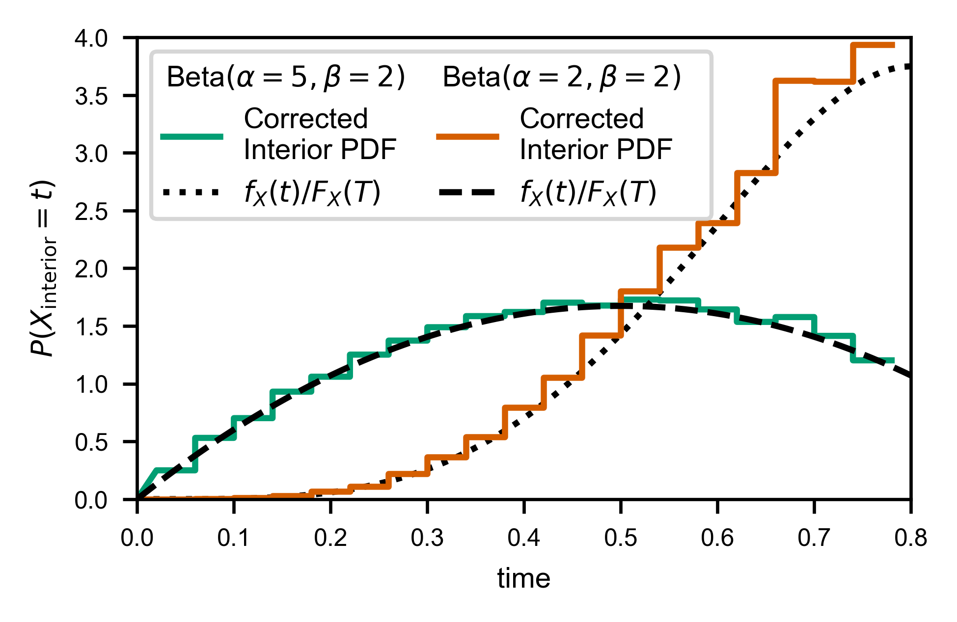
Looks like it works as well as one could hope….

fig, ax = plt.subplots(
    figsize=figure_size['full column'],
    constrained_layout=True
)

legend_entries = {var.name: [mpl.patches.Patch(alpha=0, label=var.pretty_name)]
                  for var in wait_vars}
T = discrete_waits.window_size.max()
for var in wait_vars:
    interior = discrete_waits.loc[
        (discrete_waits['state'] == var.name) & (discrete_waits['wait_type'] == 'interior'),
        ['wait_time', 'window_size']
    ]

    # don't need to bin to create histogram, since we measure only a discrete set of times
    x, cdf = fw.ecdf_windowed(
        interior.wait_time.values,
        interior.window_size.values,
        times_allowed=movie_frame_t
    )
    # deals with empty final bin, shifting bins over by half a dt, prepending the zero, etc.
    X, Y = fw.bars_given_discrete_cdf(x, cdf)
    line, = ax.plot(X, Y, c=var.color, label='Corrected\nInterior PDF')
    legend_entries[var.name].append(line)

    t = np.linspace(0, T, 100)
    line, = ax.plot(t, var.pdf(t)/var.cdf(T),
                    c='k', ls=var.linestyle, label=f'$f_X(t)/F_X(T)$')
    legend_entries[var.name].append(line)

ax.set_xlabel('time')
ax.set_ylabel(r'$P(X_\mathrm{interior} = t)$')
ax.set_xlim([0, T])
ax.set_ylim([0, 4])
handles = [h for _, patches in legend_entries.items() for h in patches]
legend = ax.legend(handles=handles, ncol=2, columnspacing=0.5)

# hack to left-align my "fake" legend column "titles"
for vpack in legend._legend_handle_box.get_children():
    for hpack in vpack.get_children()[:1]:
        hpack.get_children()[0].set_width(0)
# even after the hack, need to move them over to "look" nice
legend.get_texts()[0].set_position((-40/600*mpl.rcParams['figure.dpi'], 0))
legend.get_texts()[3].set_position((-40/600*mpl.rcParams['figure.dpi'], 0))

Theoretical Details

The following section contains a complete derivation of the framework used to generate the corrections used in this module.

Motivating (A)synchronicity

We first motivate our definition of “(a)synchronicity”, the critical property that allows us to correct for the effects of observing in a finite window.

Suppose a process starts at :math:-t_\text{inf} (WLOG, assume it starts in state :math:A). For times after :math:-t_\text{inf} \lll 0, the process switches between states :math:A and :math:B. The distribution of times spent in each state before switching are IID, and distributed like :math:f_A(t) and :math:f_B(t), respectively. We then are able to observe the process during the interval of time :math:[0, T].

from IPython.core.display import SVG
SVG(filename='./images/waiting-time-base-diagram.svg')

This can be thought of as a renewal(-reward) process that started far in the past. As long as the starting point, :math:-t_\text{inf}, is sufficiently far in the past, and the distributions :math:f_*(t) have finite variance, various convenient properties hold true for the observed state switching times between :math:0 and :math:T. We use the same example as in the “tutorial” section in what follows.

import scipy.stats
from multi_locus_analysis import finite_window as fw
e44 = scipy.stats.expon(scale=4, loc=4)
e16 = scipy.stats.expon(scale=6, loc=1)
trajs = fw.ab_window([e44.rvs, e16.rvs], window_size=20, offset=-1000,
    num_replicates=10000, states=['exp(4,4)', 'exp(1,6)'])

The first convenient property is that the switching times are uniformly distributed within the observation interval (as :math:-t_\text{inf}\to-\infty). Intuitively, this just means that :math:-t_\text{inf} is far enough in the past that, independently of the distribution, we are not biased towards the switching times being early or late in our observation interval (i.e. we have lost all memory of the “real” start time).

plt.figure(figsize=[4,3])
plt.hist(trajs['start_time'].values, 100)
plt.xlim([0, 20])
plt.xlabel('Rate of "creation of left ends"')

Now let’s label the observed state switches as :math:t_0,\ldots{},t_{n-1}, with :math:t_0 and :math:t_n corresponding to the “actual” (unobserved) state switch times flanking the observation interval. The next useful property is that the start of the observation interval (:math:t=0) is uniformly distributed within :math:[t_0, t_1] (similarly, the end of the observation interval, :math:t=T, is uniformly distributed in :math:[t_{n-1}, t_n].

plt.figure(figsize=[4,3])
t01 = trajs[trajs['start_time'] < 0]
u = -t01['start_time']/(t01['end_time'] - t01['start_time'])
plt.hist(u, 100)
plt.xlabel('Fraction of way between state changes at $t=0$.')

For the interior times, we can simply use the first fact to derive our interior time correction. Since we know the starting times of each state are uniformly distributed, we immediately can tell that if a waiting time of length \(\tau\) has a start time within the interval, then the the fraction of times that this waiting time will end up being an interior time is just \((T - \tau)/T\). More precisely, we have that

\[P(t_{i+1} \leq T | t_{i+1}-t_i=\tau, t_i \in [0,T]) = \int_0^T 1_{t_i + \tau \leq T} f_{\text{Unif}[0,T]}(t_i) dt_i\]

which is just equal to :math:(T - \tau)/T.

This correction factor can be visualized easily as simply counting what fraction of “start” times of a given length lead to “end” times still inside the interval. Namely, it’s the green part of the interval in the following diagram:

:width: 400

:alt: pictoral demonstration of equation above

On the other hand, we have to be careful about the distribution of exterior times, even if we do somehow magically have the values of :math:t_0 and the state at :math:t=0. You can’t simply assume that :math:t_1 - t_0 is distributed like :math:f_A(t) or :math:f_B(t). After all, in fact it is distributed like :math:tf_*(t). This is because (loosely speaking) if you fill the real line with a bunch of intervals whose lengths are distributed like :math:f(t), then you choose a point on the real line at random, you are more likely to land in an interval of size :math:t the longer that :math:t is.

plt.figure(figsize=[4,3])
a1 = t01[t01['state'] == 'exp(4,4)']
x, cdf = fw.ecdf(a1['end_time'] - a1['start_time'])
kernel = fw.smooth_pdf(x, cdf)
plt.plot(x, kernel(x), label=r'$\hat{f}(t)$: Observed CDF of $t_1 - t_0$')
plt.plot(x, e44.pdf(x), label=r'$f(t)$: Actual CDF of exp(4,4)')
Z = scipy.integrate.quad(lambda x: x*e44.pdf(x), 0, np.inf)
plt.plot(x, x*e44.pdf(x)/Z[0], label=r'$t f(t)/\int_0^\infty t f(t) dt$')
plt.legend()

(A)synchronicity

While the explicit framework presented above is a useful tool, it is ill-defined for heavy-tailed processes, in which we are primarily concerned when making these types of corrections. In order to retain the useful properties of the system that made it possible to derive the interior and exterior times distributions, we simply notice that the real property that we want to be true when measuring these systems is asynchronicity, or what a physicist might call “symmetry under time translations” or “time homogeneity”. In short, we want to impose the constraint that we are only interested in scientific measurements where changing the interval of observation :math:[0, T] to :math:[0+\tau,T+\tau] for any :math:\tau will not change any properties of the measurement.

We leave as an exercise to the reader to show that:

1. the renewal process of the previous section is a special case of an asynchronous process
2. this definition of asynchronicity produces all three properties we demonstrated for our renewal process above

On the other extreme from asynchronicity is the situation in which the Meier-Kaplan correction was originally designed to be used. Namely, we could imagine that a perfectly synchronous process is one where :math:t_0 is fixed to be at time :math:t=0, meaning that :math:t_1 - t_0 is distributed as just :math:f_*(t).

While in principle anything between asynchrony and synchrony is possible, it is true in general that almost all scientific measurements area already done using either purely synchronous or asynchronous systems, since it is intuitively clear that a lack of understanding of the synchronicity of one’s system can lead to uninterpretable results.