Analytical theory
Here, we show some best practices for comparing MSDs, displacement distributions, and velocity correlations to the theory of diffusing molecules.
The literature contains many good reviews on these topics, so we cover only some often overlooked pitfalls.
First, we review the most-used model of viscoelastic diffusion (for both free molecules and large polymers).
The first common pitfall we address is the effect of confinement on MSDs, especially on extracting diffusivity and the subdiffusivity coefficient (i.e. Hurst index).
Then, we discuss the effects of heterogeneity between measurements on the gaussianity of the displacement distribution and what that looks like for real data.
Finally, we discuss how to use the velocity cross correlation of two particles to extract information about whether those two particles are connected (such as by being on the same polymer) using a drift-independent approach.
Modeling viscoelastic diffusion
The crowded cellular environment is often subdiffusive, and across bacteria, in some yeast and some higher mammalian cells, it has been shown that this diffusion is well described by a fractional Brownian motion (for example, see (Weber et. al., PRL, 2010)).
A particle undergoing fractional Brownian motion can be modeled by a fractional Langevin equation (ignoring inertial terms)
where we use the usual Caputo definition of the fractional derivative \(\partial_t^\alpha\). This corresponds to a power-law memory kernel, \(K(t-t_0) = \frac{(2-\alpha)(1-\alpha)}{|t - t_0|^\alpha}\), where
replaces the constant viscosity of the regular Langevin equation
Intuitively, this means that there is a viscoelastic force that tries to return the particle to it’s original location (by opposing the historical velocity of the particle). The strength of this force falls off as \(t^{-\alpha}\).
The right-hand side of this equation is called the “Brownian force” and is a gaussian process with mean zero and covariance determined by the fluctuation-dissipation theorem
The viscoelastic memory kernel is parameterized by the single parameter \(\alpha\), which describes how much the system wishes to return (elastically) to a previous configuration.
The simplest way to incorporate the effects of being on a polymer is to use the Rouse model for polymer dynamics. This model is a formal way to describe how a so-called “Gaussian chain” (i.e. the limit as the number of beads goes to infinity of a model where the polymer is composed of beads \(X_i(t)\) connected by springs) behaves when undergoing thermal fluctuations.
where \(b\) is called the “Kuhn length” of the Gaussian chain, and describes (for a fixed time) how changing the length of the polymer changes the volume occupied by the polymer.
While the Gaussian chain (and by proxy, the Rouse model) is often unrealistic for isolated, short polymer chains, it can be shown mathematically (for example, see the section on Gaussian chains in Doi and Edwards) that every polymer has a Kuhn length, and behaves identically to a Gaussian chain on long enough length scales. Therefore, for the case of two loci on chromatin, separated by more than a couple of kilobases, we argue that the Rouse model is more than sufficient.
Note
Notice that this equation is very reminiscent of the Fokker-Planck-Kolmogorov equation for continuous time random walk (CTRW).
A the probability distribution for the position of a free particle undergoing a CTRW where the step sizes are Gaussian and the waiting times between steps are distributed like \(\hat{\phi}(s) = 1/(1 + 1/\hat{\eta}(s))\) (where the hat denotes a Laplace transform), can be modeled via
In the case where \(\eta\) is a power law (like \(t^{1-\alpha}\)), this reduces to our Langevin equation above, with the Brownian force removed.
These equations are fundamentally different however, because in our model the fluctuation dissipation theorem connects the Brownian force \(F_B\) to the viscosity. This means the velocity correlation for a fBm particle is given by \(\langle V(t) V(0) \rangle \propto -t^\alpha\), whereas since the CTRW takes independent steps by construction, and so has \(\langle V(t) V(0) \rangle = 0\) almost everywhere.
In what follows, we consider the diffusion to be well described by a simple fractional Brownian motion, with no random waiting times between collisions. The combination of these two models ((f)Bm and a CTRW) is discussed to some degree in the Supplemental Materials of (Beltran and Kannan, PRL 2019), and represents well a random walk with heavy-tailed “defects”.
MSDs
The MSD of a particle diffusing according to the equations above can be written as
In other words, in log-log space, the MSD will be a line with slope \(\alpha\).
Note
While this is true even for arbitrarily short times in our fractional diffusion model (due to its fractal nature), for real particles diffusing in actual viscoelastic materials (like beads in a polymer gel), as we probe shorter and shorter times, there should be a time scale on which the elastic forces of the material are not felt. At these size scales in real data we will often see an MSD that looks like a regular diffusion (a line with slope \(\alpha = 1\) in log-log space). At even shorter times (usually too short to measure), the particle will eventually exhibit ballistic behavior, as it travels processively between collisions between the molecules that surround it.
If we instead consider the diffusion of a polymer instead of a point, we get a new equation of motion. See [WTS10] for a complete derivation.
In short, what we find is that the observed MSD in log-log space will be a line with slope \(\alpha/2\) for short time scales. This persists until the terminal relaxation time \(t_R = [N^2b^2\xi/(k_BT)]^{1/\alpha}\) of the polymer, which is the time scale at which the polymer as a whole can be said to be diffusing (in other words, the time scale at which the diffusion of the center of mass of the polymer begins to dominate over the internal fluctuations of the polymer). At times scales longer than the terminal relaxation time, the MSD will be a line with slope \(\alpha\), and the polymer as a whole will diffuse as if experiencing an effective viscosity of \(N\xi\).
>>> import matplotlib as mpl
>>> from multi_locus_analysis import analytical
>>> alpha = 0.8; N = 100; b = 1
>>> t = np.logspace(-6, 6, 100)
>>> msd = analytical.rouse_mid_msd(t, alpha, b, N, num_modes=1000)
>>> plt.loglog(t[t>1], 3/N*np.sin(alpha*np.pi)/(
>>>     np.pi*(1-alpha/2)*(1-alpha)*alpha)*np.power(t[t>1], alpha),
>>>     '-.', label=r'$\propto t^\alpha$')
>>> plt.loglog(t, np.power(t, alpha/2), '-.', label=r'$t^{\alpha/2}$')
>>> plt.loglog(t, msd, 'k', label='MSD(t)')
>>> plt.xlabel('time (AU)')
>>> plt.ylabel(r'MSD ($\mu{}m^2$)')
>>> plt.legend()
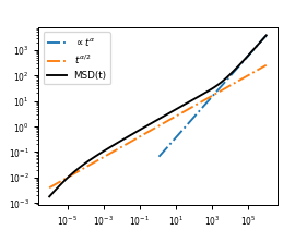
Note that the drop-off on the left-hand side of the MSD plot is simply due to
the finite number of Rouse modes included when numerically evaluating the MSD.
The Rouse polymer is a “fractal” model, so the proper solution to the equations
of motion presented above has an MSD whose short-time behavior scales as
\(t^{\alpha/2}\) indefinitely. The log of the number of modes included
(optional arg num_modes in the call) corresponds exactly to the number of
orders of magnitude that will have the correct scaling in the calculated MSD.
However, this drop-off is also instructive, because this fractal behavior is exactly the most unrealistic part of the Rouse model. In real systems, at short enough time scales, a monomer on the polymer will also transition back to the background slope of \(\propto\alpha\). This means that if you measure an actual locus on a polymer, say a particular locus of a small plasmid in a mammalian cell (where \(\alpha\approx 1\)). Then we will see a curve that looks just like the black curve above. The long time crossover (from \(t^{\alpha/2}\) to \(t^\alpha\)) will measure the terminal relaxation time of the plasmid (the time scale after which diffusion of a locus on the plasmid is dominated by diffusion of the plasmid as a whole). The short crossover time (from \(t^\alpha\) to \(t^{\alpha/2}\)) will correspond to the time scale at which thermal forces from the surrounding medium begin to be dominated by the elastic restoring force from the polymer chain.
Note
The fractional Brownian motion itself is also a fractal model, and as such has the similar shortcomings to the Rouse model. Namely, at long enough time scales, if confinement isn’t a factor, it is likely that the MSD will transition eventually to a slope of \(\alpha=1\) for any realistic system. This may also be true for short enough times. In a sense, what one can say is that the fBm Rouse model is really telling us is that for the time scales described above, whatever the medium value of \(\alpha\) is, being on a polymer simply halves it. Thus it is always important to compare polymer MSDs to the MSD of a free particle in the same medium, since many complex mediums will not have a single characteristic value of \(\alpha\), but instead have an MSD whose slope depends on the time or length scale (e.g. due to defects or traps of a particular size scale). If comparison to a free particle is not possible experimentally, there are also other ways to estimate the terminal relaxation time of the polymer if this is not possible (see velocity cross correlation discussion below).
So in experimental MSDs, where the chromosomal loci are confined to a given spatial region (whether that be a chromosome territory or the nucleus as a whole), we expect to see the MSD curve cut off at a different location depending on how the confinement time scale compares to the terminal relaxation time of the chromosome (or chromosomes, if they are linked together).
Hopefully it can be surmised from this discussion that even for this simplest possible model of Rouse polymer motion, simply fitting MSD curves with straight lines in log-log space can lead to extremely misleading results, due to the non-linear nature of the MSD curve itself. Therefore, it is important to establish the confinement diameter, and terminal relaxation time of the polymer at a minimum, before trying to fit a raw MSD to extract, for example, a value for \(\alpha\).
Displacement Distributions
The paper of Lampo et al is extremely valuable for understanding how heterogeneity in diffusivities between different cells can lead to a population that appears to have a non-guassian displacements distribution even though each underlying cell may itself have gaussian displacements.
A more general overview of the combined effects of intra-cellular and inter-cellular heterogeneity can be found in the later paper by Stylianidou and Lampo.
In short, while both the fractional and classical Rouse models assume Gaussian step sizes between time steps, we observe significantly heavier tails in the displacement distributions in vivo. The two papers above discuss how this might be the product of there being significant heterogeneity in the diffusivity of the polymer.
Velocity Cross-Correlation
In order to measure whether (and how) stress is communicated between the loci being measured, we can look at their velocity cross correlation functions.
The velocity autocorrelation of a free particle undergoing fractional Brownian motion will serve as a useful comparison throughout what follows in order to understand limiting behavior of the more complicated, polymer case. Such a particle has a velocity autocorrelation function given by
where we should notice that \(C_v^{(\delta)}(0)\) is just the MSD as a function of \(\delta\). We plot this function below for a few values of \(\alpha\).
>>> td = np.linspace(0, 4, 401)
>>> betas = np.concatenate([np.linspace(0, 1, 6), np.array([1.5, 2])])
>>> betas[0] += 0.0001
>>> cmap = plt.get_cmap('viridis')
>>> cnorm = mpl.colors.Normalize(vmin=0, vmax=1.5)
>>> for beta in betas:
>>>     label = f'$\\beta = {beta:0.1}$' if beta < 1 else f'$\\beta = {beta}$'
>>>     plt.plot(td, analytical.frac_discrete_cv_normalized(td, 1, beta),
>>>              label=label, c=cmap(cnorm(beta)))
>>> plt.xlabel(r'$t/\delta$')
>>> plt.ylabel(r'$C_v^{(\delta)}(t)$')
>>> plt.legend(loc='upper right')
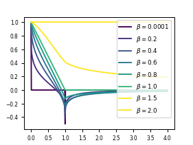
Notice that as \(\alpha\) goes to 1, the velocity correlation goes to that of a regular Brownian motion, \(\max\{1 - t/\delta, 0\}\). As \(\alpha\) goes to 2, the velocity correlation becomes identically 1 (as expected for ballistic motion). As \(\alpha\) goes to 0, the velocity correlation is identically zero, with unit spikes at zero and one in the positive and negative directions, respecitvely (as expected for totally arrested motion).
As shown in (Lampo & Spakowitz, Biophysical Journal, 2016), the velocity cross-correlation of two loci on a Rouse polymer can be computed exactly.
after a cosine transform in \(n\), and expanding in the eigenbasis of the fractional derivative, \(E_{\alpha,1}\) (the Mittag-Leffler functions), we get
The first term captures the motion of the center of mass of the polymer, while the terms in the sum capture the motion due to different “modes” of the polymer.
The coefficients \(k_p = \frac{3\pi^2k_BT}{Nb^2} p^2\) then determine how strongly to weight each mode as a function of \(t\) and \(\delta\).
Because \(E_{\alpha,1}(x)\to 0\) as \(x\to-\infty\), and since \(k_p \propto p^2\), the summation converges fairly quickly. However, using the numerical values for \(\phi_p(n_i)\) tends to cause numerical instabilities. Instead, we consider several limiting cases where properties of the cosine function allow us to simplify the expression. For example, if we simply want to compute the polymer locus’s autocorrelation function, then \(n_1 = n_2\), which gives us Eq. 33 of (Weber & Spakowitz Physical Review E, 2010).
Infinite Polymer Limit
In the simple, but typical case where \(\alpha = 1\), the infinite polymer case becomes significantly simpler than the general case of a finite polymer.
We can express the velocity correlation of two loci on an infinite polymer in a regular viscous medium in terms of the Meijer G-functions, which are defined as the Mellin-Barnes integrals
For two loci separated by a distance \(\Delta n\), the correlation function is simply given by
This function can be evaluated exactly using any numerical library that has routines for evaluating Meijer G-functions. In particular, in Python, this functionality is implemented in the well-tested package mpmath.
Velocity Cross-Correlation “Trick”
Let us consider the velocity autocorrelation of the distance between two monomers \(C_{\Delta{}V}^{(\delta)}\), where \(\Delta{}V^{(\delta)}(t) = \Delta X(t + \delta) - \Delta X(t)\) and \(\Delta X(t) = X_2(t) - X_1(t)\).
This quantity has the useful property of being drift-free. That is, an arbitrary rotation and translation can be applied to the sample at each time without affecting the values of \(\Delta{}V^{(\delta)}(t)\).
It is simple enough to notice that this is simply equal to
where the monomer velocity autocorrelation \(C_{v}^{(\delta)}(t)\) and the velocity cross correlation between two monomers \(C_{vv}^{(\delta)}\) is as above.